Field line following and Poincaré maps#

This page describes the FieldLine diagnostic available in pyrokinetics. This diagnostic allows the user to follow perturbed magnetic field lines in gyrokinetic simulations and compute quantities such as:

Poincaré maps
radial diffusion coefficients
radial displacement
magnetic field correlation lengths
field line tearing parameter (linear)

These diagnostics are particularly useful for analysing magnetic stochasticity and transport in nonlinear gyrokinetic simulations.

The diagnostic operates by integrating the perturbed magnetic field along a magnetic field line using the fluctuating parallel vector potential \(A_{||}\) obtained from the simulation output.

This functionality is available through the class pyrokinetics.diagnostics.field_line.FieldLine.

Basic usage#

First we import pyrokinetics and create a Pyro object for the simulation we want to analyse.

import numpy as np
import matplotlib.pyplot as plt

from pyrokinetics import Pyro, template_dir
from pyrokinetics.diagnostics.field_line import FieldLine

fname = template_dir / "outputs/CGYRO_nonlinear/input.cgyro"
pyro = Pyro(gk_file=fname, gk_code="CGYRO")

pyro.load_gk_output()

Next we define the initial positions of the magnetic field lines we want to follow. These are given in the flux-tube coordinates \((x,y)\).

xarray = np.linspace(6, 8, 5) * pyro.norms.rhoref
yarray = np.linspace(-10, 10, 3) * pyro.norms.rhoref

We also specify:

the number of poloidal turns
the time slice of the simulation
the value of \(\rho_*\)

nturns = 1000
time = 1
rhostar = 0.036

Now create the diagnostic object and compute the field line trajectories.

diag = FieldLine(pyro)
coords = diag.follow_field_line(xarray, yarray, nturns, time, rhostar)

The result is an array containing the coordinates of each field line intersection:

shape = (2, nturns, len(yarray), len(xarray))

where

coords[0] is the radial coordinate \(x\)
coords[1] is the binormal coordinate \(y\)

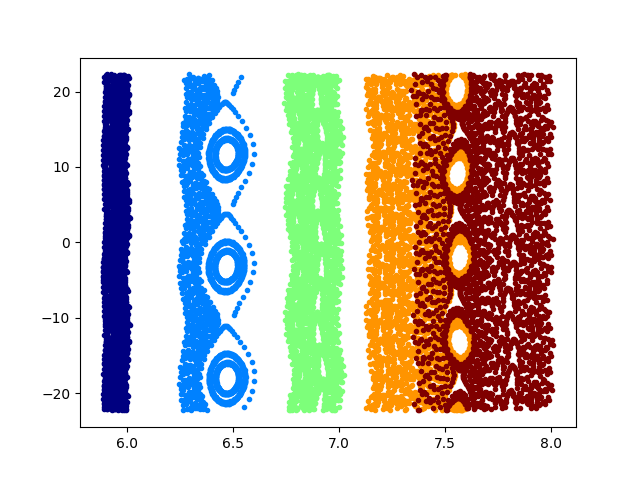
Plotting a Poincaré map#

A Poincaré map can be generated by plotting the successive intersection points of the field line with a poloidal plane.

colorlist = plt.cm.jet(np.linspace(0, 1, xarray.shape[0]))

plt.figure()

for i, color in enumerate(colorlist):
    plt.plot(
        coords[0, :, :, i].ravel().m,
        coords[1, :, :, i].ravel().m,
        ".",
        color=color,
    )

plt.xlabel("x")
plt.ylabel("y")
plt.show()

These maps can be used to visualise magnetic island structures and stochastic magnetic field regions.

Field line integration#

The field line trajectories are computed by integrating the perturbed magnetic field components along the equilibrium field line.

The displacement of the radial coordinate \(x\) along the field line is given by

\[\Delta x = \Delta \theta \frac{\delta \mathbf{B}\cdot\nabla x} {\mathbf{B}\cdot\nabla\theta}\]

The perturbed magnetic field can be written as

\[\delta \mathbf{B} = \delta B^x a_x + \delta B^y a_y + \delta B^\theta a_\theta\]

Since

\[\delta \mathbf{B}\cdot\nabla x = \delta B^x\]

we only need the radial component of the perturbed magnetic field.

Magnetic field from the vector potential#

The perturbed magnetic field is obtained from the curl of the vector potential:

\[\delta B^x = \frac{1}{J_{xy\theta}} \left( \frac{\partial \delta A_\theta}{\partial y} - \frac{\partial \delta A_y}{\partial \theta} \right)\]

\[\delta B^y = \frac{1}{J_{xy\theta}} \left( \frac{\partial \delta A_x}{\partial \theta} - \frac{\partial \delta A_\theta}{\partial x} \right)\]

Assuming the \(\theta\) derivatives are negligible

\[\frac{\partial}{\partial\theta} \rightarrow 0\]

this becomes

\[\delta B^x = \frac{1}{J_{xy\theta}} \frac{\partial \delta A_\theta}{\partial y}\]

\[\delta B^y = -\frac{1}{J_{xy\theta}} \frac{\partial \delta A_\theta}{\partial x}\]

Parallel vector potential#

The gyrokinetic simulations provide the parallel vector potential

\[A_{||} = \delta \mathbf{A} \cdot \hat{b}\]

where

\[\hat{b} = \frac{a_\theta}{\sqrt{g_{\theta\theta}}}\]

so that

\[A_{||} = \frac{\delta A_\theta}{\sqrt{g_{\theta\theta}}}\]

Substituting this into the expressions for the magnetic field gives

\[\delta B^x = \frac{\sqrt{g_{\theta\theta}}}{J_{xy\theta}} \frac{\partial A_{||}}{\partial y}\]

\[\delta B^y = -\frac{\sqrt{g_{\theta\theta}}}{J_{xy\theta}} \frac{\partial A_{||}}{\partial x}\]

Using Fourier modes

\[\partial_y \rightarrow -i k_y\]

we obtain

\[\delta B^x = -i \frac{\sqrt{g_{\theta\theta}}}{J_{xy\theta}} k_y A_{||}\]

Final field line equation#

Using the identity

\[\mathbf{B}\cdot\nabla\theta = \frac{d\psi}{dr}\frac{1}{J_{r\alpha\theta}}\]

and

\[C_y = \frac{1}{B_{ref}} \frac{\partial\psi}{\partial r}\]

the radial displacement becomes

\[dx = -\frac{i k_y}{B_{ref}} \int d\theta \sqrt{g_{\theta\theta}} A_{||}\]

This is the quantity integrated numerically in the code to determine the field line trajectory.

Additional diagnostics#

The FieldLine class also provides several additional diagnostics.

Field line tearing parameter#

For linear gyrokinetic simulations, the radial displacement of a magnetic field line over one poloidal turn can be used to identify microtearing modes (MTMs). These modes produce a finite radial shift of magnetic field lines associated with reconnection driven by the parallel vector potential \(A_{||}\).

The compute_linear_tearing_parameter diagnostic estimates the net field-line deviation over a poloidal circuit using the parallel vector potential structure along the field line.

The returned quantity is a dimensionless tearing parameter defined as the ratio of the net displacement to the total excursion along the field line.

Field line distance element#

In field-aligned coordinates the differential length along the magnetic field line is determined by the field-aligned covariant metric element

\[g_{\theta\theta}\]

The infinitesimal distance travelled along the field line is therefore

\[dl = \sqrt{g_{\theta\theta}} \, d\theta\]

where \(\theta\) is the poloidal angle.

Weighted field-line displacement#

The parallel vector potential \(A_{||}\) determines the magnetic perturbation responsible for magnetic reconnection. To estimate the net field line deviation over one poloidal turn we consider the quantity

\[A_{||} \sqrt{g_{\theta\theta}}\]

which weights the magnetic perturbation by the physical length element along the field line.

Integrating this along the field line gives the total signed displacement

\[\Delta = \int A_{||}(\theta)\sqrt{g_{\theta\theta}} \, d\theta\]

However, since \(A_{||}\) can change sign along the field line, a useful measure of the net tearing displacement is obtained by normalising the signed integral by the total magnitude of the excursion:

\[T = \frac{\left| \int A_{||}(\theta)\sqrt{g_{\theta\theta}} \, d\theta \right|} {\int \left|A_{||}(\theta)\sqrt{g_{\theta\theta}}\right| d\theta}\]

This dimensionless quantity

\[0 \le T \le 1\]

measures how coherent the magnetic perturbation is along the field line.

Physical interpretation#

\(T \approx 0\)

The perturbation changes sign frequently along the field line and the net displacement cancels. This is typical of electrostatic or non-tearing modes.
\(T \approx 1\)

The perturbation maintains a coherent sign along the field line, producing a finite radial displacement per poloidal turn. This behaviour is characteristic of microtearing modes (MTMs).

Thus the tearing parameter provides a convenient way to identify microtearing activity in linear gyrokinetic simulations.

Implementation#

The algorithm performs the following steps:

Extract the parallel vector potential

apar = gk_output["apar"].isel(kx=0, ky=0, time=-1)

Restrict the domain to the symmetric ballooning region.
Compute the field-aligned metric component

\[g_{\theta\theta}\]
Reconstruct the metric over the ballooning domain.
Form the weighted perturbation

\[A_{||}\sqrt{g_{\theta\theta}}\]
Integrate along \(\theta\) using Simpson integration.

The tearing parameter is then computed numerically as

apar_dl = apar * np.sqrt(g_theta_theta)

tearing_parameter = abs(
    simpson(apar_dl, x=theta)
) / simpson(
    abs(apar_dl), x=theta
)

This diagnostic is particularly useful for automatically detecting microtearing behaviour in linear parameter scans.

Radial diffusion coefficient#

The radial diffusion coefficient can be computed using

D_r = diag.radial_diffusion_coefficient(
    xarray,
    yarray,
    nturns,
    time,
    rhostar,
)

This is obtained from the mean square radial displacement of the field lines.

Radial displacement#

The average radial displacement along the field line can be computed using

delta_r = diag.compute_half_displacement(
    xarray,
    yarray,
    time,
    rhostar,
)

Magnetic field correlation length#

The parallel correlation length of the magnetic field fluctuations can be computed with

lambda_Bxx = diag.parallel_correlation_length(time)

This quantity is computed using the Wiener–Khinchin theorem and the power spectrum of the magnetic field fluctuations.

Summary#

The FieldLine diagnostic provides a flexible way to study magnetic field structure in gyrokinetic turbulence simulations. It enables analysis of:

stochastic magnetic field topology
magnetic island formation
radial magnetic transport
correlation properties of magnetic fluctuations
field line tearing parameter (linear)

These tools are particularly useful for understanding magnetic stochasticity and its contribution to transport in magnetised plasmas.

Field line following and Poincaré maps

Contents