Ideal ballooning solver

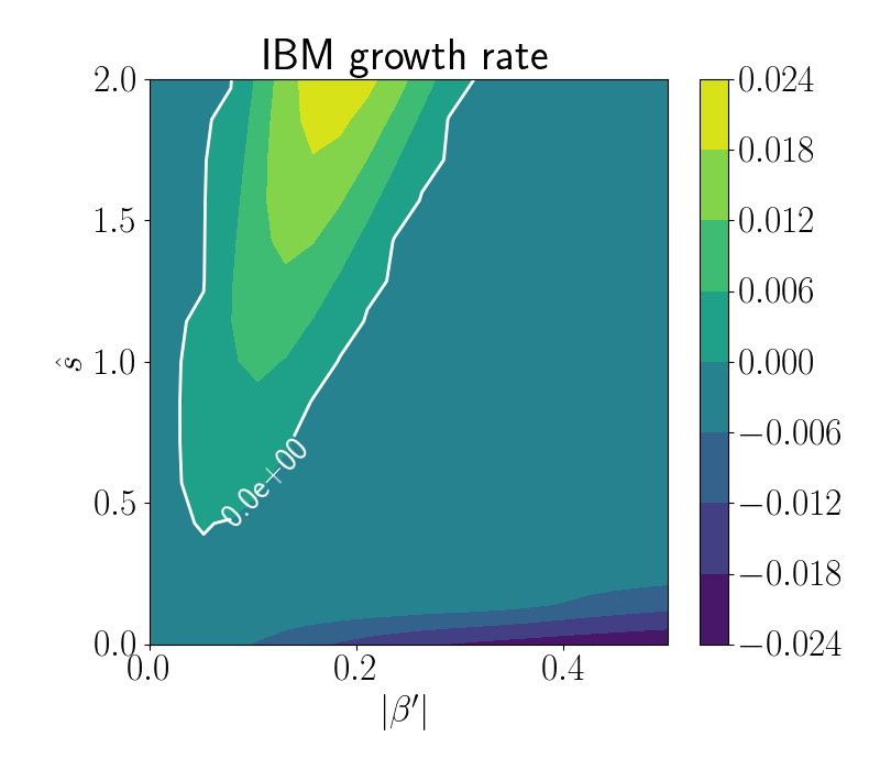
This example runs the ideal ballooning solver in pyrokinetics for a range of \(\hat{s}\) and \(\beta\) and plots this data

import numpy as np
import matplotlib.pyplot as plt
from pyrokinetics import Pyro
from pyrokinetics.diagnostics import Diagnostics
from pyrokinetics import template_dir

nshat = 15
nbprime = 20
shat = np.linspace(0.0, 2, nshat)
bprime = np.linspace(0.0, -0.5, nbprime)

pyro = Pyro(gk_file=template_dir / "input.gs2")

gamma = np.empty((nshat, nbprime))

for i_s, s in enumerate(shat):
    for i_b, b in enumerate(bprime):
        pyro.local_geometry.shat = s
        pyro.local_geometry.beta_prime = b
        diag = Diagnostics(pyro)
        gamma[i_s, i_b] = diag.ideal_ballooning_solver()


fig, ax = plt.subplots(1, 1, sharex=True, figsize=(8, 7))

cs = ax.contourf(abs(bprime), shat, gamma)
cs_0 = ax.contour(
    abs(bprime),
    shat,
    gamma,
    colors="w",
    linewidths=(2,),
    levels=[
        0.0,
    ],
)

ax.clabel(cs_0, fmt="%.1e", colors="w", fontsize=22)
ax.set_ylabel(r"$\hat{s}$")
ax.set_xlabel(r"$|\beta'|$")
fig.colorbar(cs)
ax.set_title("IBM growth rate")
fig.tight_layout()
plt.show()

This would generate the following figure

Note this works for any pyro object independant of the LocalGeometry chosen.

The algorithm used to solve the ideal ballooning equation was taken from ideal-ballooning-solver