Reading and plotting linear outputs

The following discusses how one is able to obtain and visualise data from linear gyrokinetic simulations within pyrokinetics.

We first need to load in our data from the desired directory using a Pyro object. Using GS2 as our example code:

from pyrokinetics import Pyro, template_dir

# Point to GS2 input file
gs2_template = template_dir / "outputs/GS2_linear/gs2.in"

# Load in file
pyro = Pyro(gk_file=gs2_template, gk_code="GS2")

# Load in GS2 output data
pyro.load_gk_output()
data = pyro.gk_output

Here we have loaded up the gk_output object, which is an xarray Dataset. More information about this can be obtained by printing:

>>> print(data)
<pyrokinetics.GKOutput>
(Wraps <xarray.Dataset>)
Dimensions:         (theta: 73, kx: 1, ky: 1, time: 21, field: 1, species: 2,
                                    energy: 8, pitch: 37, flux: 3)
Coordinates:
  * time            (time) float64 0.0 1.01 2.02 3.03 ... 17.17 18.18 19.19 20.2
  * kx              (kx) float64 0.0
  * ky              (ky) float64 0.07
  * theta           (theta) float64 -9.425 -9.25 -9.076 ... 9.076 9.25 9.425
  * energy          (energy) float64 0.004047 0.1044 0.5516 ... 4.739 5.936 7.25
  * pitch           (pitch) float64 0.003676 0.01921 0.04652 ... 1.182 1.194
  * species         (species) <U8 'ion1' 'electron'
  * field           (field) <U3 'phi'
  * flux            (flux) <U8 'particle' 'heat' 'momentum'
Data variables:
    phi             (theta, kx, ky, time) complex128 [([tref] / [mref])**(0.5) * [mref] / [bref_B0])·tref_electron/e/lref_minor_radius] ...
    particle        (field, species, ky, time) float64 [([tref] / [mref])**(0.5)·([tref] / [mref])**(0.5) * [mref] / [bref_B0])²·nref_electron/lref_minor_radius²/rad] ...
    heat            (field, species, ky, time) float64 [([tref] / [mref])**(0.5)·([tref] / [mref])**(0.5) * [mref] / [bref_B0])²·nref_electron·tref_electron/lref_minor_radius²/rad] ...
    momentum        (field, species, ky, time) float64 [([tref] / [mref])**(0.5) * [mref] / [bref_B0])²·nref_electron·tref_electron/lref_minor_radius/rad] ...
    growth_rate     (kx, ky, time) float64 [lref_minor_radius/([tref] / [mref])**(0.5)] ...
    mode_frequency  (kx, ky, time) float64 [lref_minor_radius/([tref] / [mref])**(0.5)] ...
    eigenvalues     (kx, ky, time) complex128 [lref_minor_radius/([tref] / [mref])**(0.5)] ...
    eigenfunctions  (field, theta, kx, ky, time) complex128 [] (4.22038619873...
Attributes: (12/14)
    linear:                 True
    gk_code:                GS2
    input_file:             &kt_grids_knobs\n    grid_option = 'single'\n/\n\...
    attribute_units:        {}
    title:                  GKOutput
    software_name:          Pyrokinetics
    ...                     ...
    object_uuid:            7bb419cd-8e4d-4465-b075-8baf37c18d34
    object_created:         2023-08-07 16:47:06.639348
    session_uuid:           cba1d994-3318-4e40-8c4d-c41e042a2b3e
    session_started:        2023-08-07 16:46:59.397799
    netcdf4_version:        1.6.1
    growth_rate_tolerance:  <xarray.DataArray 'time' ()>\n<Quantity(0.0564343...

where we can see the different data variables available, including their dimensionality, coordinates and units.

To read our desired variable, we use the syntax data["Data_variable"]:

# Get eigenvalues
eigenvalues = data["eigenvalues"]
growth_rate = data["growth_rate"]
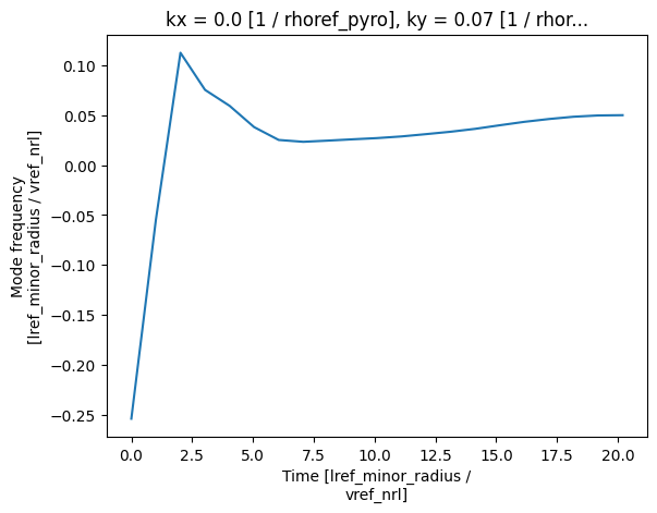
mode_freq = data["mode_frequency"]

For linear simulations, one tends to only have a single ky and kx, and thus data variables such as growth_rate and mode_frequency are essentially 1D functions of time. These can be plotted using plot (see xarray’s Plotting for further details):

mode_freq.plot(x="time")
plt.show()

For data variables with higher dimensions, indexing can be performed using the standard xarray dataset methods, such as .sel and .isel. For example, to plot the phi eigenfunction at the final time point as a function of theta:

# Plot eigenfunction
phi_eig = np.real(data["eigenfunctions"].sel(field="phi").isel(time=-1))
phi_eig.plot(x="theta", label="Real")

phi_i_eig = np.imag(data["eigenfunctions"].sel(field="phi").isel(time=-1))
phi_i_eig.plot(x="theta", label="Imag")

plt.legend()
plt.show()

Similarly for the linear fluxes, one can again specify the coordinates for the desired data. For example, to plot the electrostatic ion energy fluxes:

# Plot ion energy flux
ion_flux = data["heat"].sel(field="phi", species="ion1").sum(dim="ky")
ion_flux.plot()
plt.show()

And analogously for the field data, for example looking at the magnitude of the phi fluctuations at \(\theta = 0.0\):

# Plot phi
phi = data["phi"].sel(theta=0.0, method="nearest").isel(ky=0).isel(kx=0)
phi = np.abs(phi)
phi.plot.line(x="time")

plt.yscale("log")
plt.show()

Details regarding normalisations and units can be found in Normalisation conventions.